
1 Introduction
Seismological and geodetic observations have been carried out to understand the physical process of interplate coupling Geodetic observation is used to obtain surface deformation on East Java and surrounding area. The magnitude and distribution of interplate coupling are estimated using a geodetic inversion technique based on the formulation of Okada (1992). Seismological observation is used as constraints in the geodetic inversion. The theory of dislocations embedded in an elastic halfspace is applied in the formulation. Assuming that the
| Received, Revised, Accepted for publication |
|---|
hanging wall does not deform over the long term, an interplate coupling modeling approach is reasonable (Savage, 1983). This method assumes isotropic condition inside elastic dislocation area which means the stress at the coupling area will generate slip in the similar direction. This method is particularly compact and systematically composed of terms representing deformation in an infinite medium, a term related to surface deformation and that is multiplied by the depth of observation point (Okada, 1992). Therefore, this method is proposed to be applied in this study.
Large thrust earthquakes close to the Java trench are typically interplate faulting events along the slab interface between the Australia and Sunda plates. These earthquakes also generally have high tsunamigenic potential due to their shallow hypocentral depths. In some cases, these events have demonstrated slow momentrelease, and have been defined as 'tsunami' earthquakes, where rupture is large in the weak crustal layers very close to the seafloor. Most of the large earthquakes in Java occurred in west and east of Java. The large tsunami earthquake that has been occurred in eastern Java is the 1994 M7.8 Banyuwangi earthquake and 2006 M7.7 Pangandaran earthquake. Banyuwangi earthquake is categorized as the largest earthquake in Java for last 20 years. Banyuwangi earthquake occurred on 2nd June 1994, this event produced a tsunami with wave run-up heights of 13 m, killing over 200 people. While the tsunami of up to 15 m, and killed 730 people by Pangandaran Earthquake that occurred on 17th July 2006 was produced. While both of these tsunami earthquakes were characterized by rupture along thrust faults, they were followed by an abundance of normal faulting aftershocks. These aftershocks are interpreted to result from extension within the subducting Australia plate, while the mainshocks represented interplate faulting between the Australia and Sunda plates (USGS, 2016).
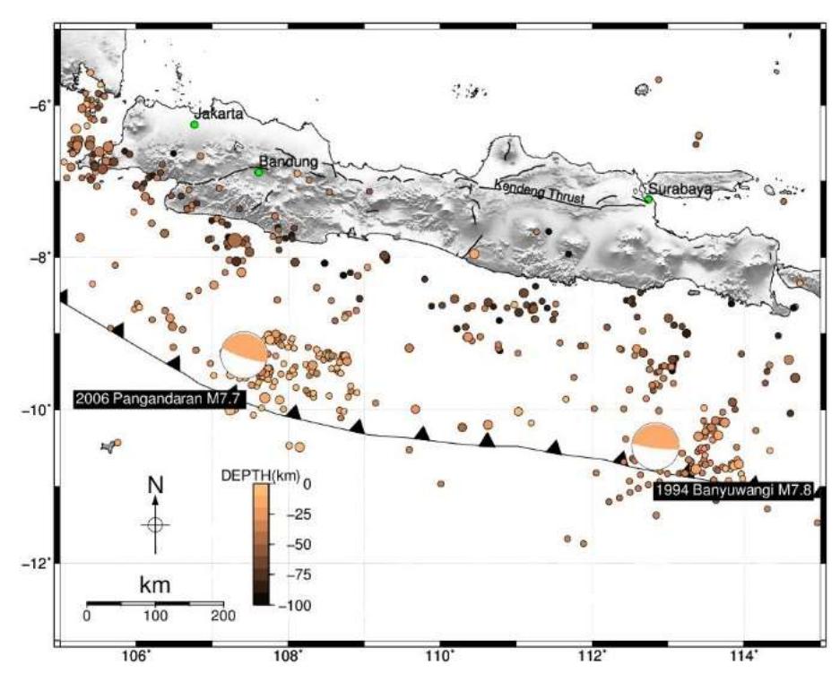
Figure 1 Seismicity activity around Java Island. The colored dot represent earthquake >5Mw and the maximum depth at 100 Km.
In figure 1 due to that matter, this research proposes the first initiation of deformation studies correlating the surface deformation around east java using GPS with the slip distribution on the convergence area. Furthermore, this method can be used in another subduction area to make comprehensive studies.
2 Material and Method
GPS Observation Data
The main objective of monitoring surface deformation is to help to predict the slip distribution on the interseismic fase. These objectives can be completed by collecting some data. There are three main data (orbit, clock, ion) used in this research. We collect two main data from Geospatial Agency of Indonesia. The first one is campaign GPS observation data that is obtained from GPS. The observation data consists of seven observation points that are located around east java and west part of bali island. The second one is fifteen continuous GPS observation that is from InaCORS Network. The 15 station is surround east of java island. The third is IGS data that is used as a reference point. There are ten
sites used in this research. Those sites. These sites are distributed uniformly around Indonesia. All of the data used in this research have a 30 second interval of data acquisition. Later, the GPS observation points around the area study will be tied to the IGS sites in order to determine their coordinates.
Research Methodology
In this research is aims to review the interseismic phase of the convergence zone around East java using surface deformation around area study. We collect the daily solution ythat free from outlier of all GPS station to generate the displacement rate that free of periodic signal. The displacement rate is using ITRF2000 and continue to reducing the effect of sunda block motion. The clean displacement rate as input for the geodetic inversion that referref to the theory of dislocations in elastic half-space. The theory is implemented by using Okada (1992) equation with the assumption that the slip vector on the coupling area is remaining parallel to the long-term interplate velocity. To estimate the value of interseismic coupling in the fault segment model, the geodetic inversion will be calculated from the data of the displacement rate of each point on land that transfer into fault model segment. A fault model for geodetic inversion is shown in Figure 2.
To perform geodetic inversion, it is necessary to define three-dimensional geometry of the megathrust (fault) based on bathymetry data, slab model (USGS, 2015) and deformation model of Australian Plate (Bock et. al., 2015). In order to obtain a high spatial resolution of interplate coupling, fault geometry is defined with nodes every 25 km and smoothly interpolated along width and strike. The fault geometry data and visualization are shown in Table 1 and Figure 3 respectively.
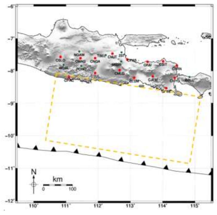
Figure 2 The fault model (yellow dashed line). The red colored dot is refer to Continuous GPS and Green colored dot is refer to campaign GPS
Figure 3 Ilustration of 3 dimensional geometry of megathrust (Meilano, 2014)
| Parameter | Value | Refference |
| 279.9920 | Slab model (USGS, | |
| Strike (φ) | 2015) | |
| 0 | Slab model (USGS, | |
| Dip (δ) | - 300 4 | 2015) |
| Rake (λ) | 2700 | Bock et.al., 2003 |
| Slab model (USGS, | ||
| Top Depth | 8 km | 2015) |
| Width (W) | 250 km | Defined from Data |
| Nodes (Patch sizee) | 25 km | Defined from Data |
Table 1 Three dimensional geometry of fault segment parameters
The relationship between observed surface deformation and normal slip can be described in equation (1).
\[y = Gb \tag{1}\]
Where is observed surface deformation, is normal slip on the coupling area of each sub-fault (nodes), and is Green's function, which here is a function of the parameterization of fault geometry, such as strike, dip, length, depth and location of the fault. The Green's function is calculated using the dislocation theory in the elastic half-space (Okada, 1992). If the unknown parameter is the normal slip (b), then the equation (1) can be expressed as equation (2) below.
\[b = [G^T G]^{-1} G^T y \tag{2}\]
To perform the model resolution of the model, we conduct Checker Board Test procedure. From the CBT process, we can determine the resolution test shows that the appropriate spatial resolution is the function of the distance of fault patch to the observation station.
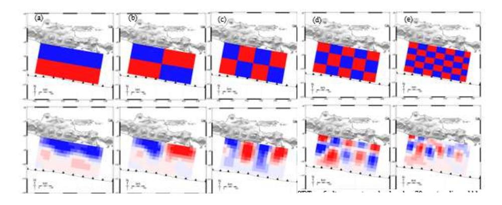
Figure 4 Checker Board Test with different patch
Spatial resolution for the shallow part (less than 30 km) is ~250 km in length and ~125 km in width, for the middle part of the deeper section (30-70 km) is better than 75 km x 50 km. The slip rate is reasonably resolved up to ~200 km from the coast, corresponding to the slab depth of 50-90 km, within a fault size until 75 km x 50 km (Figure 4 d). The model cannot resolve patches smaller than 75 km x 50 km (Figure 4 e). Resolution for the shallow part (depth < 20km) and the periphery of the source region is very limited although we may be able to distinguish the existence of a slip deficit in the shallow part by enlarging the fault size (Hanifa, 2014).
3 Result and Discussion
Displacement by GPS Observation
From the observartion GPS data, the daily solution of each site is from GLOBK generated to estimation the surface deformation. We reffered the surface deformation to sunda block motion to have the effect of convergence zone. Form those displacement rate on the land, we transfer to estimate the slip of the intraplate zone by geodetic inverion from dislocation theory in half space by okada as result in Figure 5 below.
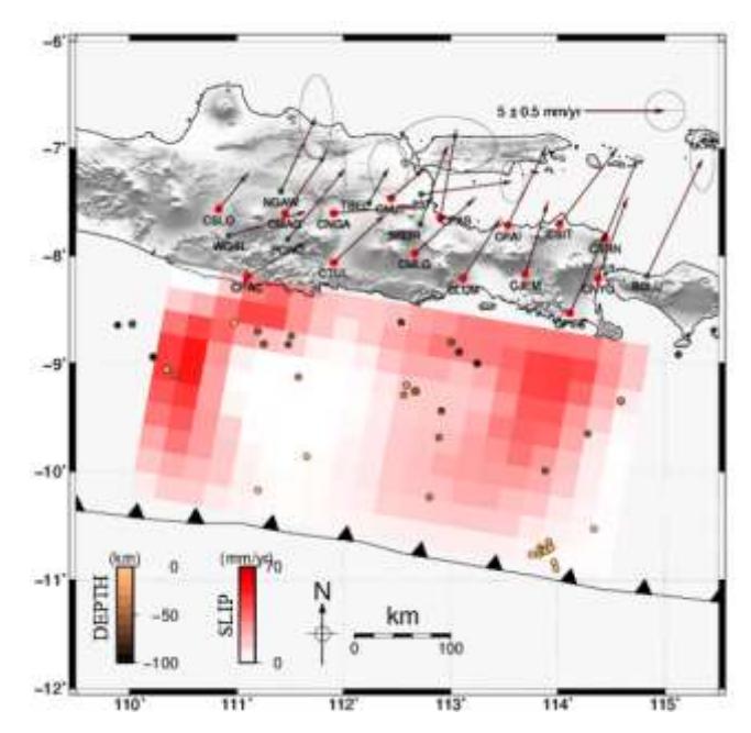
Figure 5 The Interseismic slip distribution in East Java. Red colored patch is show the value of slip and the blak to copper colored dots is show the seismic activity during observation period.
The result from the geodetic inversion is the slip with the magnitude of interseismic slip rate variance from 0 mm/yr and maximum at 55 mm/yr with rake 270 for thrust fault. The area with 0 mm/yr slip rate value denotes that as decoupled area (shown in white color), it indicates there is no seismogenic stress accumulated on that area and it is not the significant concern for this study.
There are two regions that have the large value of interseismic slip result from the calculation, first one near the coastline of Pacitan (CPAC) and the second one at the south of Banyuwangi (CNYU) that show in figure 5 (colored red patch). From those result indicates as strong coupling area which indicates the convergence zone in the area study is locked, even partially or temporarily, accumulating seismogenic stress.
We compare the distribution of interseismic slip with the seismic activity during observation period. From the overlay figure 5 shown the strong slip distribution area have less seismic activity. The less seismic activity is due to the accumulate energy on that area. Thought there are area that have a freeslip also have less seismic activity, we conduct the forward calculation to shown the fitness of the data input and the result.
Forward Calculation
Forward calculation is conduct to determine the acceptance of confidence level which comes from the interseismic slip distribution. From the interseismic slip distribution, the horizontal and vertical crustal displacement rates are calculated. deformation vector from model nearly fit the observation. The comparison between data observation and model are shown in Figure 5 and 6. The blackcolored arrow is observation displacement rate and pink-colored arrow is the model from the forward calculation.
From 22 observation station, there are three stations that have the largest residual (237, WGIR), All of two stations are campaign GPS, the residual may come from the uncertainty of overestimating to the value the data. However, the rest of observation station has the best fit with the model, it shows the value of rms from the residual between GPS observation with the model forward calculation is around ± 2.067 mm for horizontal component and 2.302 mm for vertical component. The less value of rms is shown fitness between the model and the observation data.
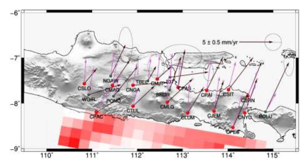
Figure 6 Comparison of displacement rate between model from forward calculation (purple coloured arrow) and observation (black coloured arrow).
4 Conclusion
This research aimed to estimate the distribution of interseismic slip in from relatively new data. Before this research was conducted, the hypothesis states that the results are expected to show the slip rate distribution as the indicator coupling area due to convergence between Indo-Australia with Sunda Block. Furthermore, the forward calculation of interseismic slip distribution will fit into surface deformation.
Based on the result and the analysis from the previous chapter, the distribution of interseismic slip in the shallow area mostly has the rake vector into the coast, which means the accumulation of deformation could be released as the rupture in the future earthquake. Those slip distribution also known as the indication of the coupled area between Indo-Australia and Sunda block. Since the large value slip on the asperity point needs to be compared to another data.
The comparison of crustal deformation between the model (from the forward calculation) and GPS observation are nearly similar for both horizontal and vertical rate shown from the RMS value of the residual. The forward calculation confirms that crustal deformation on East Java is primarily caused by Interseismic activity on the area study. However, this research found that model indicates still have the number of misfit to the observation at the GPS stations located.
5 References
- [1] Abidin, H. Z., Andreas, H., Kato, T., Ito, T., Meilano, I., Kimata, F., ... & Harjono, H. (2009). Crustal deformation studies in Java (Indonesia) using GPS. Journal of Earthquake and Tsunami, 3(02), 77-88.
- [2] Blewitt, G., Hammond, W. C., & Kreemer, C. (2005). Relating geothermal resources to Great Basin tectonics using GPS. Geothermal Resources Council Transactions, 29, 331-336.
- [3] Esposito, A., Anzidei, M., Atzori, S., Devoti, R., Giordano, G., & Pietrantonio, G. (2010). Modeling ground deformations of Panarea geothermal hydrothermal/geothermal system (Aeolian Islands, Italy) from GPS data. Bulletin of Geothermallogy, 72(5), 609-621.
- [4] Fauzi, A.,: Geothermal development in Indonesia: An Overview, Geotermia, Rev de Geoenergia, Vol 14 (3), pp. 147-152, (1998)
- [5] Floyd, M. A., & Funning, G. J. Continuation of survey GPS measurements and installation of continuous GPS sites at The Geysers, California, for geothermal deformation monitoring.
- [6] Hammond, W. C., Kreemer, C., & Blewitt, G. (2007). Exploring the relationship between geothermal resources and geodetically inferred faults slip rates in the Great Basin. Geothermal Resources Council Transactions, 31, 391-395.
- [7] Kreemer, C., Blewitt, G., & Hammond, W. C. (2006). Using geodesy to explore correlations between crustal deformation characteristics and geothermal resources. Geothermal Resources Council Transactions, 30, 441-446.
- [8] Mossop, A., & Segall, P. (1997). Subsidence at The Geysers geothermal field, N. California from a comparison of GPS and leveling surveys. Geophys. Res. Lett, 24(14), 1839-1842.
- [9] Khodayar, M., Markússon, S. H., & Einarsson, P. (2006). GPS-mapping of geothermal areas in West Iceland and tectonic interpretation.
- [10] Meilano, I. (1997). Deformasi Gunung Guntur Berdasarkan Pengamatan GPS. Undergraduate Thesis of Geodesy ITB.
- [11] PT. LAPI ITB, (2012). Kajian Prospek Panas Bumi di Daerah Jawa dan Bali. Laporan Akhir Re-Evaluasi Sistem Prospek Panas Bumi Di Daerah Jawa dan Bali. IV-20 – IV-26.